Spatially Resolved Map of M81

The following example shows how we can use Lightning to fit spatially resolved UV-to-FIR photometry (SED map) of the nearby spiral galaxy, M81.

Data

We compiled the UV-to-FIR photometry (GALEX, SDSS, 2MASS, WISE, IRAC, MIPS CH1, PACS blue and red, and SPIRE 250 and 350 \(\mu{\rm m}\)) from publicly available images, using the image processing techniques outlined in Section 2 of Eufrasio et al. (2017). These steps consisted of:

1. subtracting foreground stars,

2. convolving each image to a common \(25^{\prime\prime}\) PSF,

3. re-binning them to a common \(10^{\prime\prime}\) pixel scale,

4. estimating the background to update the photometric uncertainties,

5. correcting each bandpass for Galactic extinction,

6. combining the images into a data cube which contains the pixel-by-pixel SEDs.

We further structured the SED map data cube to have the FITS Table Format for input into Lightning. This input data file can be found in examples/map_M81/ as m81_data.fits, where the primary image extension is the key linking each SED_ID in the first extension data table to the corresponding pixel, and the table in the first extension is the Lightning formated input data.

Warning

Due to the large number of model evaluations required to fit this map with the MCMC sampler (\(5.229 \times 10^9\)) and the MPFIT minimizer (\(\approx 7.8 \times 10^7\)), we fit this example on a 32-core node of the Pinnacle cluster at the Arkansas High Performance Computing Center. The number of SED fits involved mean that storage requirements are also significant: >90 GB for the MCMC method and >10 GB for MPFIT. As such, we recommend downloading the post-processed results for each method here (or by using the download shell script: examples/map_M81/m81_postprocess_download.sh) to follow along with the example, rather than fitting the data yourself.

Configuration

For this example, we’ll configure Lightning to use Stellar Emission, the modified Calzetti Dust Attenuation, and Dust Emission models. Since we fit with both the Affine-Invariant MCMC and MPFIT algorithms, we first change the below lines of the configuration files in examples/map_M81/MCMC/ and examples/map_M81/MPFIT/ from the defaults to the configuration settings in common between the two algorithms.

Common Settings

When we run this example, we use a 32 core CPU.

MAX_CPUS: 32                                ,$

We add 5% model uncertainty

MODEL_UNC: 0.05d0                             ,$

and shrink the default initializations on the SFH, as we expect each pixel to have a small SFR.

PSI :      {Prior: ['uniform', 'uniform', 'uniform', 'uniform', 'uniform'] ,$
            Prior_arg: [[0.0d, 0.0d, 0.0d, 0.0d, 0.0d]                     ,$
                        [1.d3, 1.d3, 1.d3, 1.d3, 1.d3]]                    ,$
            Initialization_range: [[0.0d, 0.0d, 0.0d, 0.0d, 0.0d]          ,$
                                   [1.d0, 1.d0, 1.d0, 1.d0, 1.d0]]          $
            }                                                              ,$

We use the more complex modified Calzetti attenuation curve, since we have high-quality optical and IR data which may require a more flexible attenuation curve. We only change the initializations on \(\tau_{{\rm DIFF}, V}\) to smaller values, since each pixel on average should have low attenuation.

ATTEN_CURVE: 'CALZETTI_MOD'                   ,$

TAUV_DIFF: {Prior: 'uniform'                          ,$
            Prior_arg: [0.0d, 10.0d]                  ,$
            Initialization_range: [0.0d, 1.0d]         $
            }                                         ,$

As for the dust emission model, we limit initialization of \(U_{\rm min}\) and \(\gamma\) to lower values than the default, since nearby galaxies like M81 typically have \(U_{\rm min} < 5\) and \(\gamma \approx 0.01\) (Dale et al. 2017).

UMIN:    {Prior: 'uniform'                            ,$
          Prior_arg: [0.1d, 25.d]                     ,$
          Initialization_range: [0.1d, 5.0d]           $
          }                                           ,$

GAMMA:   {Prior: 'uniform'                            ,$
          Prior_arg: [0.0d, 1.0d]                     ,$
          Initialization_range: [0.0d, 0.1d]           $
          }                                           ,$

MCMC

For the MCMC algorithm configuration only (i.e., examples/map_M81/MCMC/lightning_configure.pro), we set the output file name to:

OUTPUT_FILENAME: 'm81_map_mcmc'             ,$

We then decrease the number of MCMC trials per walker to \(10^4\):

NTRIALS: 1e4                            ,$

Next, we adjust the MCMC post-processing settings to pre-defined values for the burn-in, thinning, and number of final chain elements.

BURN_IN: 8000                           ,$

THIN_FACTOR: 250                        ,$

FINAL_CHAIN_LENGTH: 250                 ,$

Finally, we reduce the definition of a stranded walker to one standard deviation below the median acceptance fraction. We found this reduction is necessary to ensure all pixels have any stranded walkers correctly classified, since an individual pixel SED is not as well behaved as a galaxy integrated SED, which we base our default value.

AFFINE_STRANDED_DEVIATION: 1.0d      $

MPFIT

For the MPFIT algorithm configuration only (i.e., examples/map_M81/MPFIT/lightning_configure.pro), we set the output file name to:

OUTPUT_FILENAME: 'm81_map_mpfit'             ,$

We then select to use the MPFIT algorithm by updating the fitting method:

METHOD: 'MPFIT'                       ,$

Finally, we slightly reduce the number of solvers to increase fitting speed.

NSOLVERS: 20                            ,$

Running Lightning

Note

The IDL code snippets below are also available in batch file format, as examples/map_M81/m81_batch.pro. The two lines explicitly for fitting, as given below, are in the file but are commented out, since fitting can take an extended period of time.

Now that we have set up the configurations, we are ready to run Lightning. However, since we only want to fit a subset of the SEDs found in m81_data.fits, let’s select the subset and save the data in a new file. First, we generate the B-band ellipse region that will define our subset of SEDs, with the ellipse shape parameters coming from the HyperLeda database.

cd, !lightning_dir + 'examples/map_M81/'

; These are the original B-band ellipse values from HyperLeda.
ra = [09, 55, 33.15]   ; units in Hour, minute, and seconds.
dec = [69, 03, 55.2]   ; units in sexagesimal degrees.
logd25 = 2.34  ; logd25 is the decimal logarithm of the length the projected major axis (d25 in 0.1 arcmin).
logr25 = 0.28  ; logr25 is the axis ratio of the isophote (decimal logarithm of the ratio of the lengths of major to minor axes).
pa = 157.0	   ; Major axis position angle in degrees (North Eastwards).

; Let's convert these values to degrees.
ra = 15 * (ra[0] + ra[1]/60. + ra[2]/3600.) 
dec = (dec[0] + dec[1]/60. + dec[2]/3600.) 
a = ((10.d^logd25 * 0.1d) /2) / 60.d  ; divide by 2 for semi-major.
q = 10.d^(-1.d * logr25)   ; axis ratio is q = b/a, negative flips ratio from major/minor to minor/major.
b = a * q                  ; semi-minor axis.

; Read in the image containing the SED_ID of each pixel and its header.
m81_map  = mrdfits('m81_data.fits', 0, hd)
; Create the ellipse mask.
bband_mask = ellipse_region(ra, dec, a, b, pa, hd)

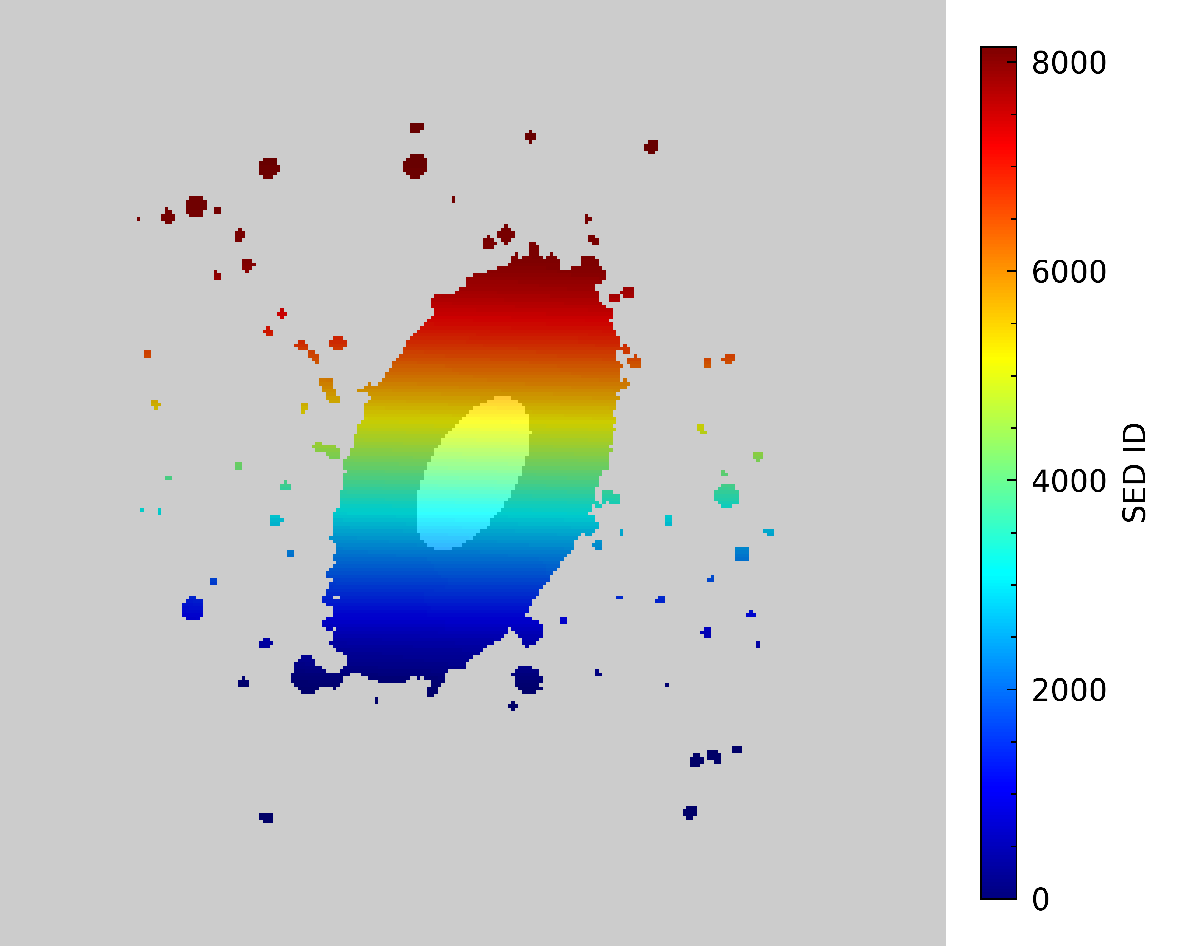
Let’s make images of the SED_ID image (m81_map) and B-band mask to make sure this worked as we expect. We will set the SED_ID image to have its pixels color coded based on the SED_ID, where any blank white area indicates pixels with no associated data, due to low SNR. As for the B-band mask, we will set pixels within the ellipse to be white and those outside to be black to help show the extent of the full image. We will then overplot it on the SED_ID map with some transparency to see how they align.

img_sed_id = image(m81_map, $
                   rgb_table=33, $
                   position=[0, 0, 0.8, 1])
cb = colorbar(target=img_sed_id, $
              orientation=1, $
              position=[0.83,0.05,0.86,0.95], $
              title='SED ID', $
              /border_on, $
              textpos=1, $
              tickdir=1, $
              font_size=12)
img_mask   = image(bband_mask, $
                   transparency=80, $
                   /overplot)

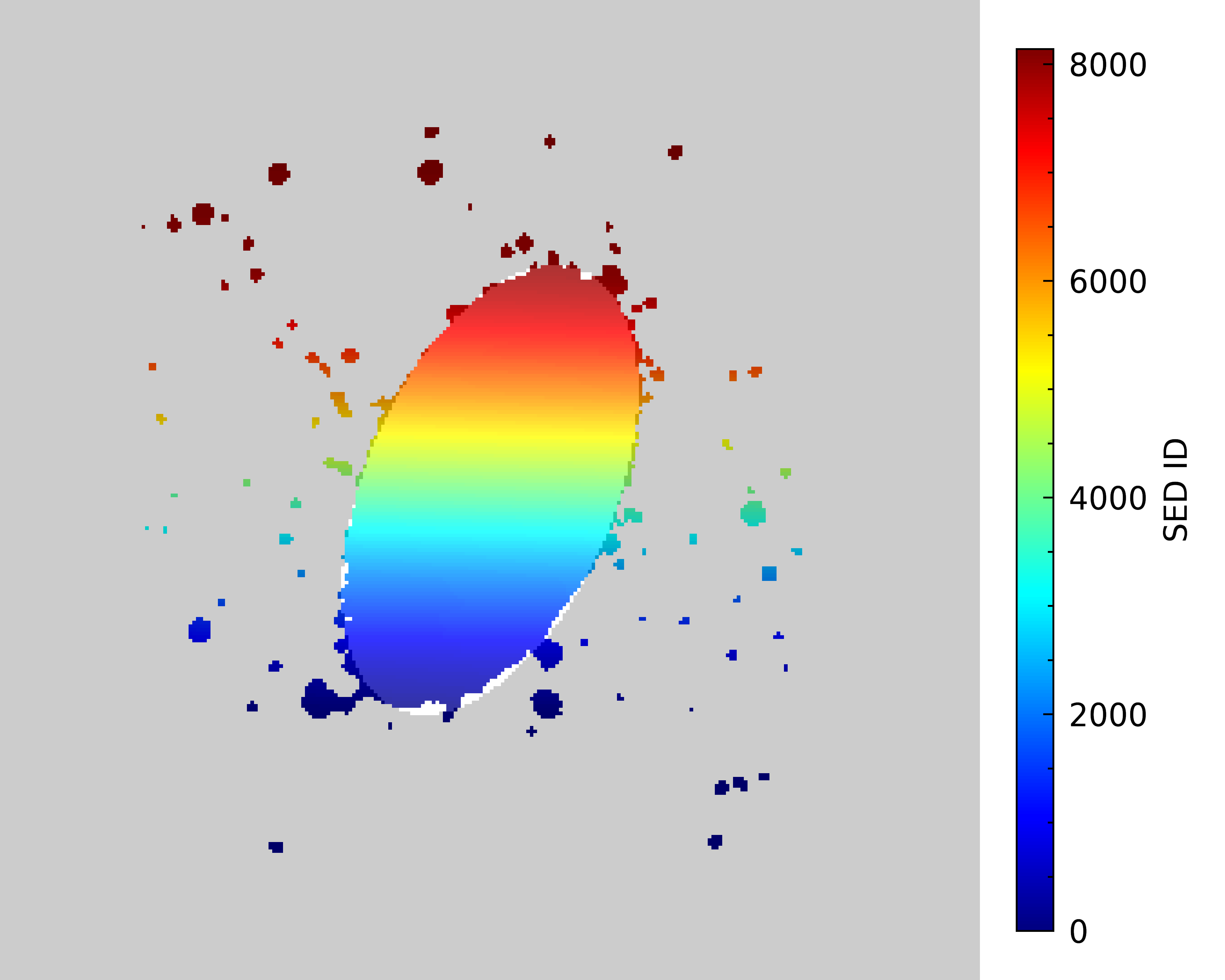
Great, our mask looks like it is covering the extent we expect. Now, we are ready to select the subset of SEDs that fall within this ellipse region.

; Read in the data table containing the SEDs.
m81_seds  = mrdfits('m81_data.fits', 1)

; We need the SED_IDs that correspond to the pixels within the mask.
; Note that we exclude any pixels that lack an SED, which is given by a NaN in m81_map.
bband_ids = m81_map[where(bband_mask eq 1 and finite(m81_map))]

; Since the SED_IDs in m81_seds are in ascending order based on value, we can just
;   index the table using the selected IDs.
fitting_data = m81_seds[bband_ids]

; Let's create individual files for the MCMC and MPFIT fittings.
mwrfits, fitting_data, 'MCMC/m81_input.fits', /create
mwrfits, fitting_data, 'MPFIT/m81_input.fits', /create

Now that we have created files containing the subset of SEDs that we want to fit, we can fit them with:

restore, !lightning_dir + 'lightning.sav'
lightning, 'MCMC/m81_input.fits'

For the MPFIT fitting, this is done with:

lightning, 'MPFIT/m81_input.fits'

Note

If you downloaded our post-processed files as recommended rather than fitting, you will need to create and place those files in the respective lightning_output directory. To simplify this for you, you can use the following IDL commands to create the directories and move the downloaded files. If you used the shell script to download the files, this steps was done for you and can be ignored.

file_mkdir, ['MCMC', 'MPFIT'] + '/lightning_output'
file_move, '<downloaded_file_path>/m81_map_mcmc.fits.gz', 'MCMC/lightning_output/'
file_move, '<downloaded_file_path>/m81_map_mpfit.fits.gz', 'MPFIT/lightning_output/'

Analysis

Convergence

Once the fits finish, Lightning will automatically create post-processed files for us containing the results. The first thing we should always do with any fit is to check it for convergence. Since we have thousands of fits (one for each pixel), we will use the Convergence Metrics and Goodness of Fit Outputs to check the quality of our results, focusing first on the MCMC fits.

; Read in the post-processed data table.
results = mrdfits('MCMC/lightning_output/m81_map_mcmc.fits.gz', 1)

; Let's check how many fits, if any, did not reach convergence by all our metrics.
print, '//Convergence Checks//'
print, 'Number with failed convergence flag: ', strtrim(total(results.convergence_flag), 2)

//Convergence Checks//
Number with failed convergence flag: 5609.00

Unfortunately, a majority of the SEDs did not reach our base definition of convergence. However, this does not mean that convergence was not reached. As discussed in the Convergence Metrics and Goodness of Fit Outputs, this flag includes both the autocorrelation time metric and the acceptance fraction. Let’s separate these out to see if one is causing more problems than the other.

; These totals count the number of SEDs with the corresponding flags set.
;   The < operator sets any value > 1 from the first total to 1.
;   This allows us to see the number of SED with an issue vs all flags.
print, '//Detailed Convergence Checks//'
print, 'Number with failed autocorrelation flag: ', strtrim(total(total(results.autocorr_flag, 1) < 1), 2)
print, 'Number with failed acceptance flag: ', strtrim(total(total(results.acceptance_flag, 1) < 1), 2)

//Detailed Convergence Checks//
Number with failed autocorrelation flag: 0.00000
Number with failed acceptance flag: 5609.00

This is good! We have no SEDs with autocorrelation times above our threshold. Instead, the issue is that at least one walker per SED has an acceptance fraction below 20%. As discussed for the affine invariant MCMC Convergence Metrics, this is not a problem. It just means that we are likely not sampling as efficiently as we could be. As recommended, let’s check if we flagged all of these low (< 20%) acceptance fractions as stranded walkers.

; This counts the number of SEDs with an acceptance flag set when the corresponding
;   stranded flag is not.
print, '//Stranded Walker Check//'
print, "Number of walkers with low acceptance fractions that /weren't/ flagged as stranged: ", $
       strtrim(total(total((results.acceptance_flag - results.stranded_flag) > 0, 1) < 1), 2)

//Stranded Walker Check//
Number of walkers with low acceptance fractions that /weren't/ flagged as stranged: 2921.00

Okay, as we can see, a good portion of SEDs did not have all of their low acceptance rate walkers flagged as stranded. This means that these 2921 SEDs actually have overall low acceptance fractions (< 20%). Let’s see if we can better visualize what is happening by plotting the median acceptance fraction of each SED versus the number of walkers per SED below our 20% acceptance threshold.

; Let's include the 1 standard deviation of the acceptance fraction, since
;   it is what is used to flag stranded walkers.
plt = errorplot(total(results.acceptance_flag, 1)/75, $
                median(results.acceptance_frac, dim=1), $
                stddev(results.acceptance_frac, dim=1), $
                linestyle='', $
                symbol='o', $
                xtitle='Fraction of walkers below 20% acceptance threshold', $
                ytitle='Acceptance Fraction')
plt = plot(plt.xrange, $
           [0.2, 0.2], $
           color='red', $
           linestyle='--', $
           thick=2, $
           /overplot)

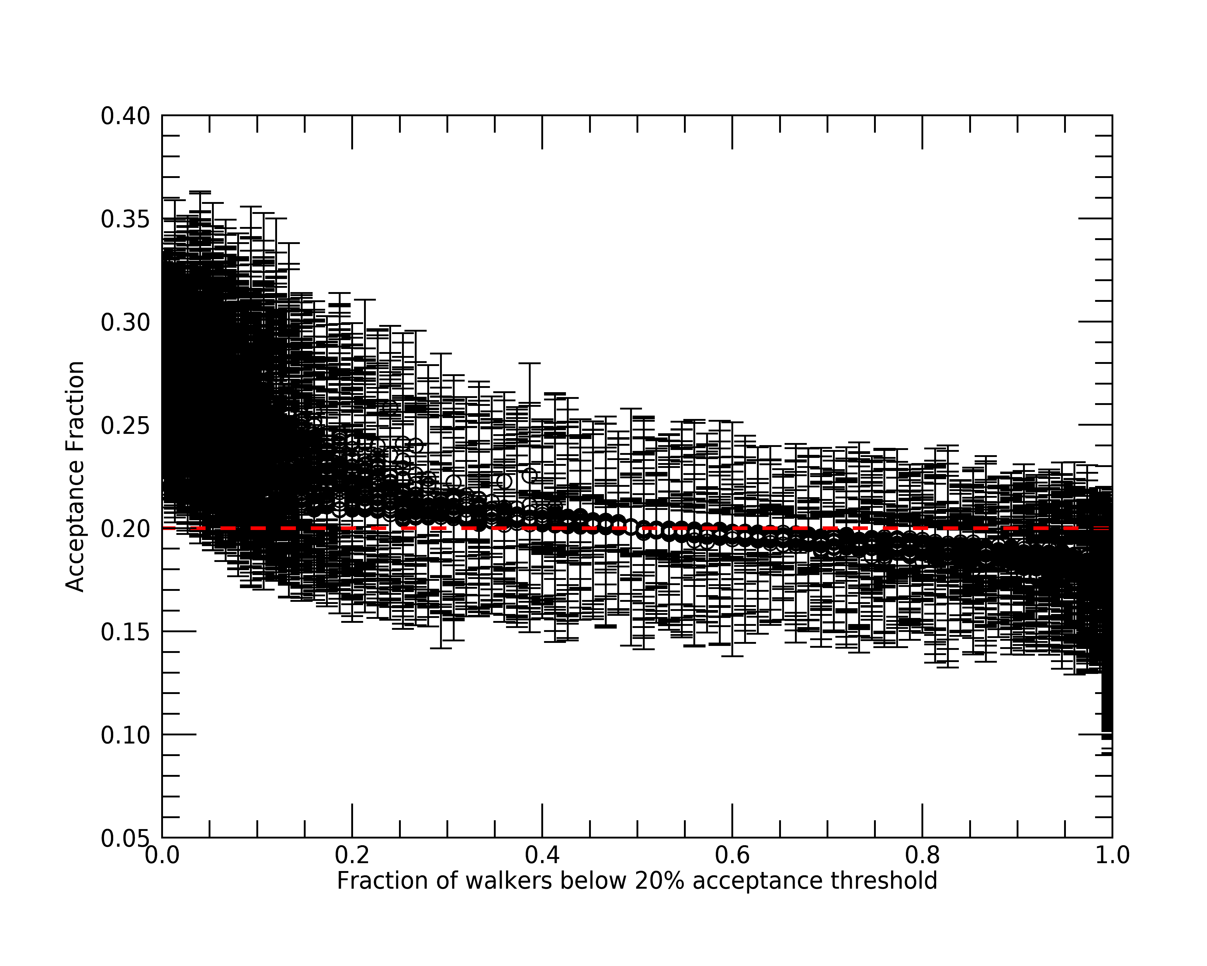
As we can see from this plot, fits with lower median acceptance fractions have more walkers flagged for having low acceptance rates as we would expected. More importantly though, the fits with the largest number of flagged walkers have median acceptance fractions mainly between 15% and 20% with standard deviations similar to fits with few flagged walkers. Therefore, since these fractions are close to 20% and the autocorrelation times indicate convergence, we can be confident that convergence was reached for these 2921 SEDs with low acceptance fractions, but not as efficiently as the rest.

Note

We could lower our AFFINE_A configuration setting to sample more efficiently for these SEDs, but due to the long duration it takes to fit all of these SEDs, we will not pursue this change.

Now that we have confirmed our MCMC results converged, lets do the same for the MPFIT results.

; Read in the MPFIT post-processed data table.
results_mpfit = mrdfits('MCMC/lightning_output/m81_map_mpfit.fits.gz', 1)

; Let's check how many fits, if any, did not reach convergence by all our metrics.
print, '//Convergence Checks//'
print, 'Number with failed convergence flag: ', strtrim(total(results_mpfit.convergence_flag), 2)

//Convergence Checks//
Number with failed convergence flag: 3568.00

So around half of our MPFIT fits did not converge based on all our metrics. Just like the MCMC results, let’s separate the metrics and see if one is indicating non-convergence more than the others.

; These totals count the number of SEDs with the corresponding flags set.
print, '//Detailed Convergence Checks//'
print, 'Number with failed status flag: ', strtrim(total(total(results_mpfit.status_flag, 1) < 1), 2)
print, 'Number that reach max iterations: ', strtrim(total(total(results_mpfit.iter_flag, 1) < 1), 2)
print, 'Number with < 50% of solvers near lowest chisqr: ', strtrim(total(results_mpfit.stuck_flag), 2)
print, 'Number with a parameter not within 1% of lowest chisqr solver: ', strtrim(total(total(results_mpfit.similar_flag, 1) < 1), 2)

//Detailed Convergence Checks//
Number with failed status flag: 0.00000
Number that reach max iterations: 81.0000
Number with < 50% of solvers near lowest chisqr: 62.0000
Number with a parameter not within 1% of lowest chisqr solver: 3538.00

So as we can see, MPFIT never failed to run, and the ITER_FLAG and STUCK_FLAG metrics indicate very few fits had these issues. The metric that is flagged the most and indicating lack of convergence is the SIMILAR_FLAG (i.e., our non-stuck solvers had > 1% differences in solutions compared to the best-fit solver). Let’s check each of these metrics in more detail, starting with iteration metric. To do this, let’s check the maximum number of solvers per pixel that reached the maximum number of iterations. If this is a minority of solvers per fit (say < 25%), we will assume that these solvers would have been considered stuck and not worry about this metric further.

print, '//Iteration Fraction Check//'
print, 'Maximum solvers to reach iteration limit: ', strtrim(max(total(results_mpfit.iter_flag, 1)), 2)

//Iteration Fraction Check//
Maximum solvers to reach iteration limit: 4.00000

Great, so at most 4 solvers (4/20 = 20%) in a given fit reached the maximim iteration limit. Therefore, we will not consider this flag a problem.

Note

This flag could easily be prevented by increasing the configuration setting ITER_MAX to be a larger value (say 500) and rerunning. We do not do this here due to the few fits and small fraction of solvers this affected.

Next, let’s check the 62 fits that had > 50% of solvers with \(\chi^2\) not within 4 of the solver with the lowest \(\chi^2\). First, let’s see the distribution of the number of solvers that had \(\chi^2\) within 4 for these fits. If the majority are at 8–9 solvers, we will consider this okay, but not ideal as we would want a majority of solvers to reach the “same” \(\chi^2\). To check this distribution, we will need to recompute the \(\chi^2\) values per solver using the calculated p-value and degrees of freedom.

; Calculate the chi2 difference. chi2 values need to be recomputed from p-values.
;   This reconversion is very accurate as long as your chi2 is not a terrible fit (i.e., p-value = 0).
chi2 = dblarr(20, n_elements(results_mpfit))
for i=0, 19 do for j=0, n_elements(results_mpfit)-1 do $
    chi2[i, j] = CHISQR_CVF((results_mpfit[j].pvalue)[i], results_mpfit[j].dof)
chi2_diff = chi2 - rebin(reform(min(chi2, dim=1), 1, n_elements(results_mpfit)), 20, n_elements(results_mpfit))

; Determine how many solvers were below a given chi2 threshold difference from the minimum
reached_min = intarr(n_elements(results_mpfit))
for j=0, n_elements(results_mpfit)-1 do reached_min[j] = n_elements(where(chi2_diff[*, j] lt 4, /null))

; Only look at the fits with the stuck_flag set.
keep = where(results_mpfit.stuck_flag eq 1, nkeep, /null)

; Creat the distribution and plot
counts = histogram(reached_min[keep], nbins=max(reached_min)-min(reached_min[keep])+1, locations=binloc)
plt = plot(binloc, $
           counts, $
           xtitle='Number of solvers with $\chi^2 - 4 \leq \chi^2_{best}$', $
           ytitle='Counts', $
           thick=2, $
           /stair)

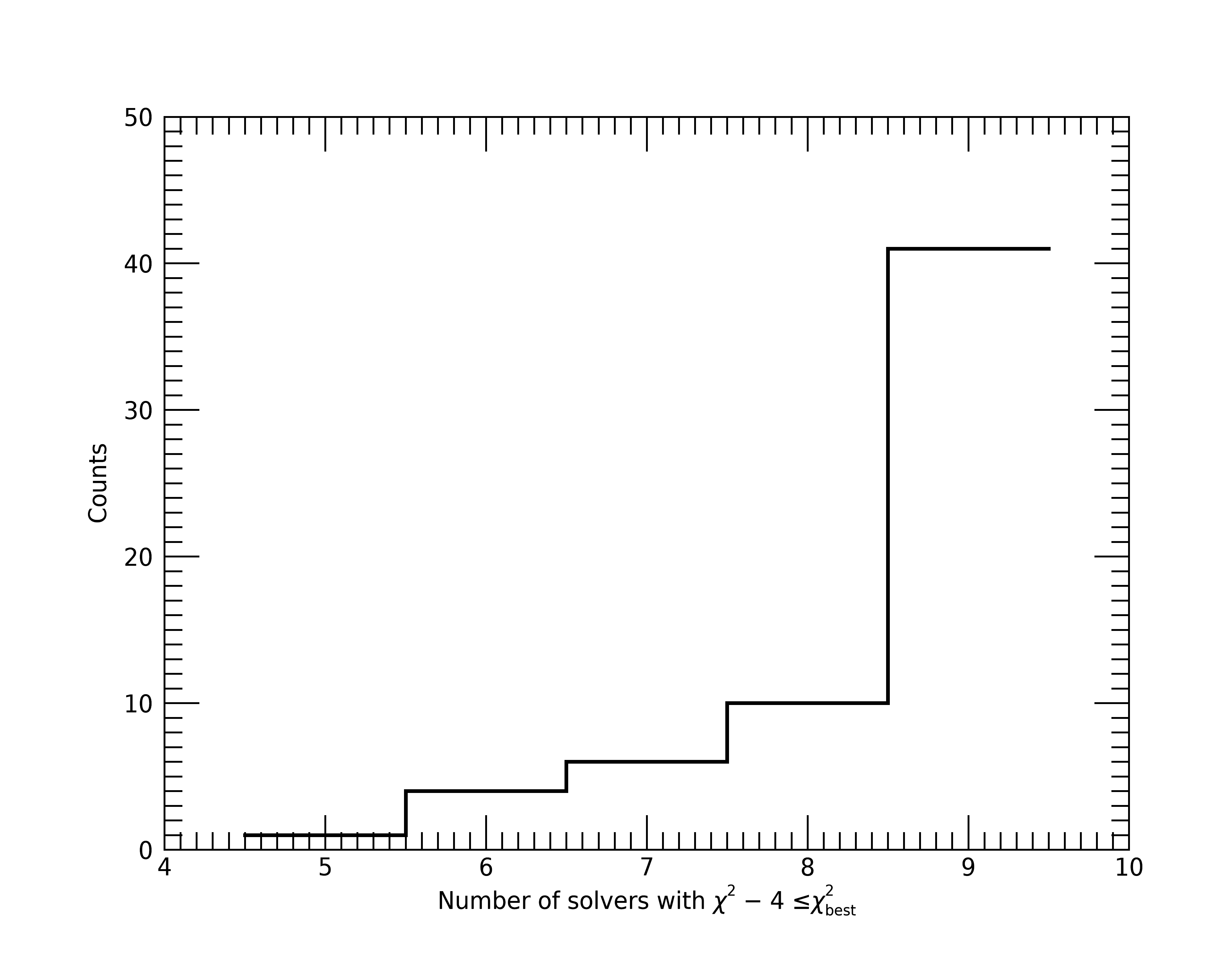
As we can see, only 10 or so fits have less than 7 solvers (but always 5+) within a \(\chi^2\) of 4 to the best solution. Therefore, we will consider this enough solvers per fit to compare parameter values for convergence (SIMILAR_FLAG).

Note

In practice, it would be best to rerun these 62 fits to attempt to get > 50% solvers near the same \(\chi^2\). This could be done by keeping the intermediate .sav files produced by the fitting algorithm (KEEP_INTERMEDIATE_OUTPUT Post-processing configuration setting) and deleting the files for the SEDs that had this issue. Then, only these deleted fits could be rerun by including the /resume keyword when Running Lightning again. We do not do this process here as we have not shared our 10 GBs of intermediate files required for a partial rerun. (We also did not have you set this configuration setting if you actual did run these fits.)

Finally, let’s compare the parameter values of the non-stuck solvers to see if 1% differences is too strict for this example. If we find the majority of solvers converged to the same solution with differences of < 5%, we can consider that convergence has occurred and that the requirement of 1% differences and all solvers converging is too strict for this example.

; Calculate the number of non-stuck solvers with similar (1, 3 and 5% difference) solutions to the bestfit
;   (if the bestfit value is 0, just use difference)
Nsimilar = dblarr(3, n_elements(results_mpfit[0].parameter_names), n_elements(results_mpfit))
for j=0, n_elements(results_mpfit)-1 do begin $
    min_loc = (where(chi2_diff[*, j] eq 0, /null))[0] &$
    bestfit_params = (results_mpfit[j].parameter_values)[*, min_loc] &$
    zero_param = where(bestfit_params eq 0, comp=nonzero_param, ncomp=Nnonzero, /null) &$
    near_min = where(chi2_diff[*, j] lt 4, Nnear_min) &$
    param_per_diff = (results_mpfit[j].parameter_values)[*, near_min] - $
                     rebin(bestfit_params, n_elements(results_mpfit[0].parameter_names), Nnear_min) &$
    if Nnonzero gt 0 then $
      param_per_diff[nonzero_param, *] = param_per_diff[nonzero_param, *] / $
                                         rebin((results_mpfit[j].parameter_values)[nonzero_param, min_loc], Nnonzero, Nnear_min) &$
    Nsimilar[0, *, j] = fix(total(fix(param_per_diff lt 0.01d), 2)) &$
    Nsimilar[1, *, j] = fix(total(fix(param_per_diff lt 0.03d), 2)) &$
    Nsimilar[2, *, j] = fix(total(fix(param_per_diff lt 0.05d), 2))

; Determine the fraction of non-stuck solvers with solutions near the bestfit
similar_frac = Nsimilar / rebin(reform(reached_min, 1, 1, n_elements(results_mpfit)), 3, 13, n_elements(results_mpfit))

; Only look at the fits with the similar_flag set.
keep = where(total(results_mpfit.similar_flag, 1) gt 0, /null)

; Check if majority of non-stuck solvers reached the same solution
solver_frac = dblarr(3, 13)
for i=0, 2 do for j=0,12 do solver_frac[i, j] = n_elements(where(similar_frac[i, j, keep] gt 0.5,/null)) / float(n_elements(keep))

print, '// Similarity fractions per parameter //'
print, 'Parameter Name 1% diff         3% diff         5% diff'
forprint, results_mpfit[0].parameter_names, solver_frac[0,*], solver_frac[1,*], solver_frac[2,*]

// Similarity fractions per parameter //
Parameter Name 1% diff         3% diff         5% diff
TAUV_DIFF      0.76257771      0.80327868      0.82193327
DELTA          0.88976824      0.92085922      0.93583947
TAUV_BC         1.0000000       1.0000000       1.0000000
UMIN           0.90474844      0.94149238      0.95845109
UMAX            1.0000000       1.0000000       1.0000000
ALPHA           1.0000000       1.0000000       1.0000000
GAMMA          0.99208593      0.99434710      0.99462974
QPAH           0.93188244      0.94318825      0.94827586
PSI_1          0.87252682      0.88863766      0.89683437
PSI_2          0.91068399      0.92340302      0.93046921
PSI_3          0.84680611      0.86715657      0.88044095
PSI_4          0.88637650      0.92085922      0.93725270
PSI_5          0.95788580      0.97201806      0.97880161

From this result, we can see that the vast majority of fits had a majority of solvers within 5% of the best fit solver. The parameter where this is the least true is \(\tau_{{\rm DIFF}, V}\). This is not unexpected, as there are bound to be multiple solutions of roughly the same \(\chi^2\), especially in optically faint areas where we may be missing data compared to brighter regions. Therefore, we consider this solution acceptable and that convergence, while not definite, is very likely reached by the vast majority of pixels in our SED map.

Figures

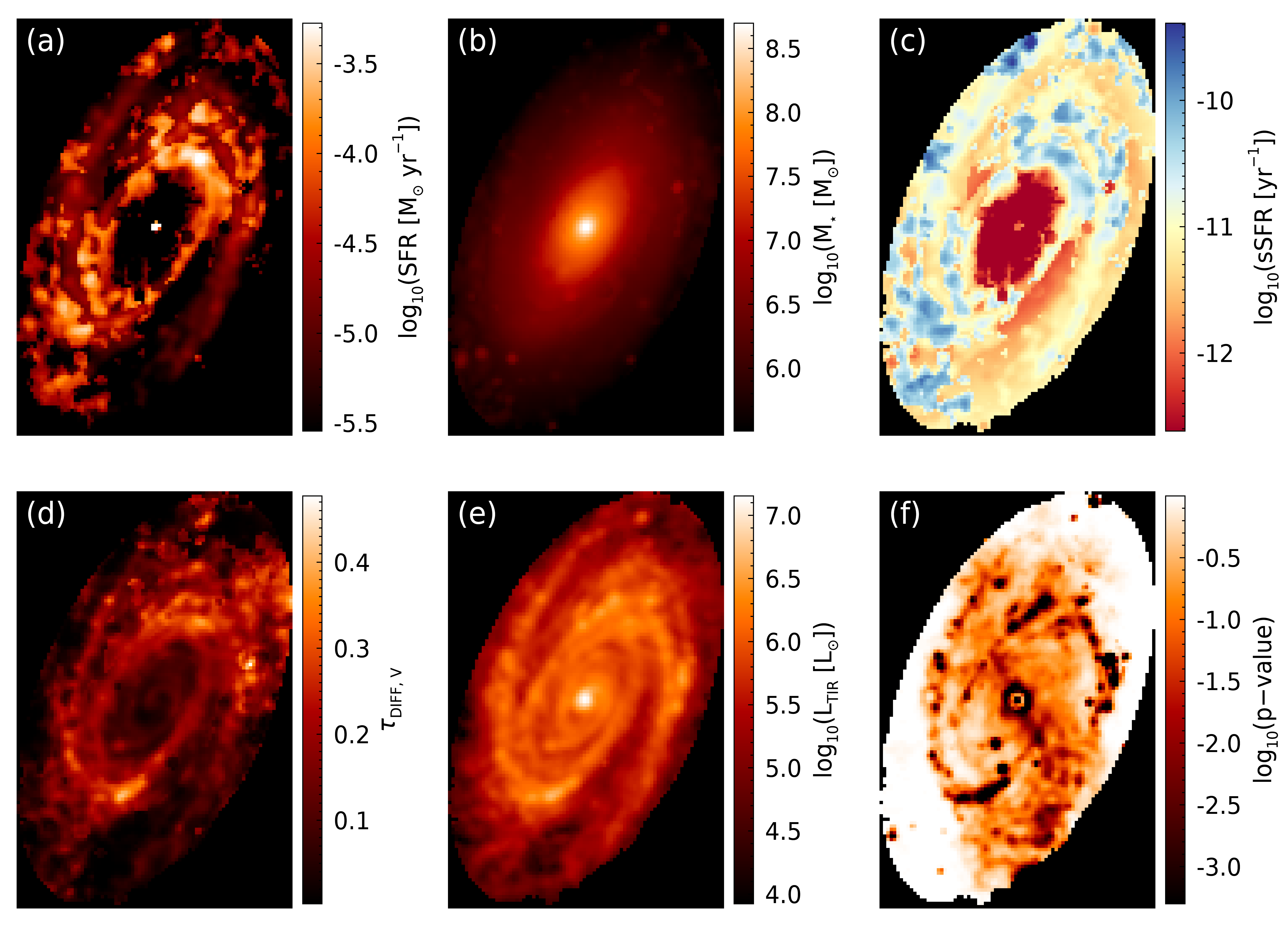
Now that we have confirmed convergence, we will make some figures to see how our results look. Let’s first make some maps of the derived physical properties. To do this, we will need to map the results from the post-processing of each SED to its associated pixel.

nsed = n_elements(results)
; Get the dimensions of the map so we can make blank ones to place our parameter values.
map_size = size(m81_map, /dim)

; We need to match each SED_ID from the result back to the map.
map_idc = lonarr(nsed)
for i=0, nsed-1 do map_idc[i] = where(m81_map eq float(strtrim(results[i].sed_id, 2)))

; Make a blank map to fill in with the results values.
sfr_map = replicate(!values.f_NaN, map_size)
; The SFR of the last 100 My is the weighted sum of the first two bins (0-10 and 10-100 Myr).
;   The bin index is the first dimension. The second dimension is the percentile values (16th, 50th, and 84th).
sfr_map[map_idc] = (results.psi_percentiles)[0, 1, *] * 0.1 + (results.psi_percentiles)[1, 1, *] * 0.9

mass_map = replicate(!values.f_NaN, map_size)
mass_map[map_idc] = median(results.mstar, dim=1)

tauv_diff_map = replicate(!values.f_NaN, map_size)
tauv_diff_map[map_idc] = median(results.tauv_diff, dim=1)

ltir_map = replicate(!values.f_NaN, map_size)
ltir_map[map_idc] = median(results.ltir, dim=1)

pvalue_map = replicate(!values.f_NaN, map_size)
pvalue_map[map_idc] = results.pvalue

Now that we have our properties maps, we can plot them. However, before we do, let’s crop them to remove the padded region surrounding the B-band ellipse as we can see in the mask image above. This will allow for better images of our data without all the extra blank space.

; Find the min and max values of where B-band mask eq 1 in each dimension.
mask_bounds_idc = minmax(array_indices(bband_mask, where(bband_mask eq 1)), dim=2)

; Crop each image to only include the B-band region.
sfr_map = sfr_map[mask_bounds_idc[0, 0]:mask_bounds_idc[1, 0], *]
sfr_map = sfr_map[*, mask_bounds_idc[0, 1]:mask_bounds_idc[1, 1]]

mass_map = mass_map[mask_bounds_idc[0, 0]:mask_bounds_idc[1, 0], *]
mass_map = mass_map[*, mask_bounds_idc[0, 1]:mask_bounds_idc[1, 1]]

tauv_diff_map = tauv_diff_map[mask_bounds_idc[0, 0]:mask_bounds_idc[1, 0], *]
tauv_diff_map = tauv_diff_map[*, mask_bounds_idc[0, 1]:mask_bounds_idc[1, 1]]

ltir_map = ltir_map[mask_bounds_idc[0, 0]:mask_bounds_idc[1, 0], *]
ltir_map = ltir_map[*, mask_bounds_idc[0, 1]:mask_bounds_idc[1, 1]]

pvalue_map = pvalue_map[mask_bounds_idc[0, 0]:mask_bounds_idc[1, 0], *]
pvalue_map = pvalue_map[*, mask_bounds_idc[0, 1]:mask_bounds_idc[1, 1]]

Let’s now plot these images!

Note

The script m81_maps.pro in the examples/map_M81/ directory generates this figure. We include this script and others associated with the complex figures to minimize the content show here, since generating these complex figures can take 100s of lines of code. Feel free to check these scripts out for our IDL plotting techniques.

; Plotting is simple with our figure script
fig = m81_maps(sfr_map, mass_map, sfr_map/mass_map, tauv_diff_map, ltir_map, pvalue_map)

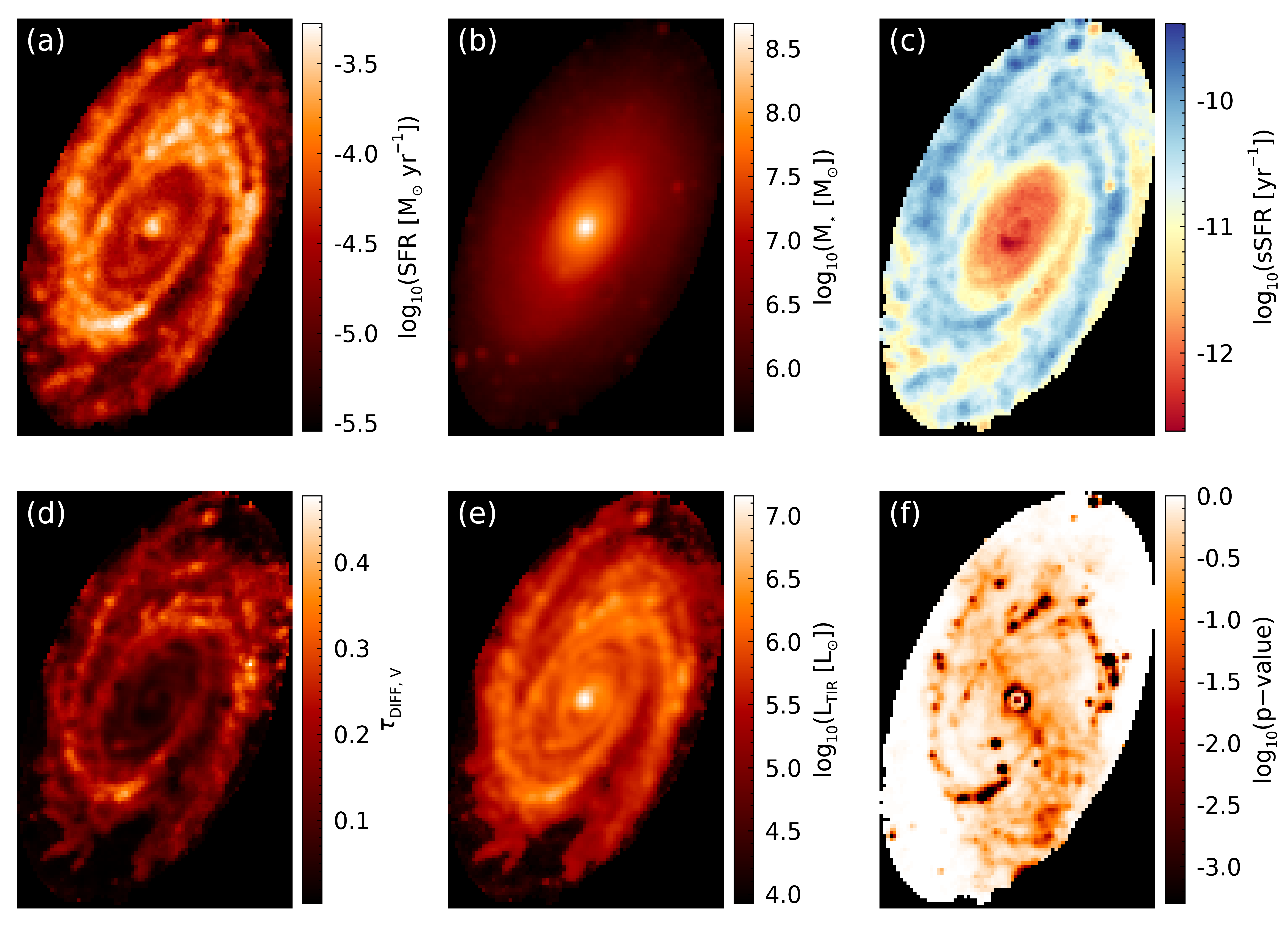
From the p-value image (panel (f)), we can see that the vast majority of pixels are well fit by our model, with poor fits mainly being associated with locations where foreground star subtraction occurred. The main take away from this figure is that spiral arms contain the younger, more highly obscured, star-forming population, while the older, less obscured, more massive population resides in the bulge region.

To show how the spatially resolved results could be used to estimate properties for regions of the galaxy, let’s separate the galaxy into two parts, an outer and inner region. We will define the outer region as the pixels between the B-band ellipse from HyperLeda and one half Ks-band ellipse from Jarrett et al. (2003). The inner region we’ll define as pixels within one half of the Ks-band ellipse. First, let’s make our one half Ks-band mask.

; Data gathered from Jarrett et al 2003.
ra = [09, 55, 33.1]     ; units in Hour, minute, and seconds.
dec = [69, 03, 54.9]    ; units in sexagesimal degrees.
r20 = 487.6   ; The length of the projected major axis at the isophotal level 20 mag/arcsec2 in the Ks-band (arcsec).
q = 0.51      ; The axis ratio of the isophote 20 mag/arcsec2 in the Ks-band (minor to major axes b/a).
pa = -31.0	  ; Major axis position angle in degrees (North Eastwards).

; Let's convert these values to degrees.
ra = 15 * (ra[0] + ra[1]/60. + ra[2]/3600.) 
dec = (dec[0] + dec[1]/60. + dec[2]/3600.) 
; Note that we use 1/2 the Ks-band 20 mag isophote
a = (r20/2.) / 3.6d3  ; semi-major axis in degrees
b = a * q             ; semi-minor axis in degrees

; Create the ellipse mask.
ksband_mask = ellipse_region(ra, dec, a, b, pa, hd)

Let’s make an image of the Ks-band mask overplotted on the SED_ID map like we did for the B-band mask.

img_sed_id = image(m81_map, $
                   rgb_table=33, $
                   position=[0, 0, 0.8, 1])
cb = colorbar(target=img_sed_id, $
              orientation=1, $
              position=[0.83,0.05,0.86,0.95], $
              title='SED ID', $
              /border_on, $
              textpos=1, $
              tickdir=1, $
              font_size=12)
img_mask   = image(ksband_mask, $
                   transparency=80, $
                   /overplot)

Great, this mask looks good. Now let’s use the two masks and our MCMC results to create some plots comparing the SEDs and SFHs of the outer and inner regions.

; Plotting is simple with our figure script
fig = m81_regions(m81_map, hd, m81_seds, results, bband_mask, ksband_mask)

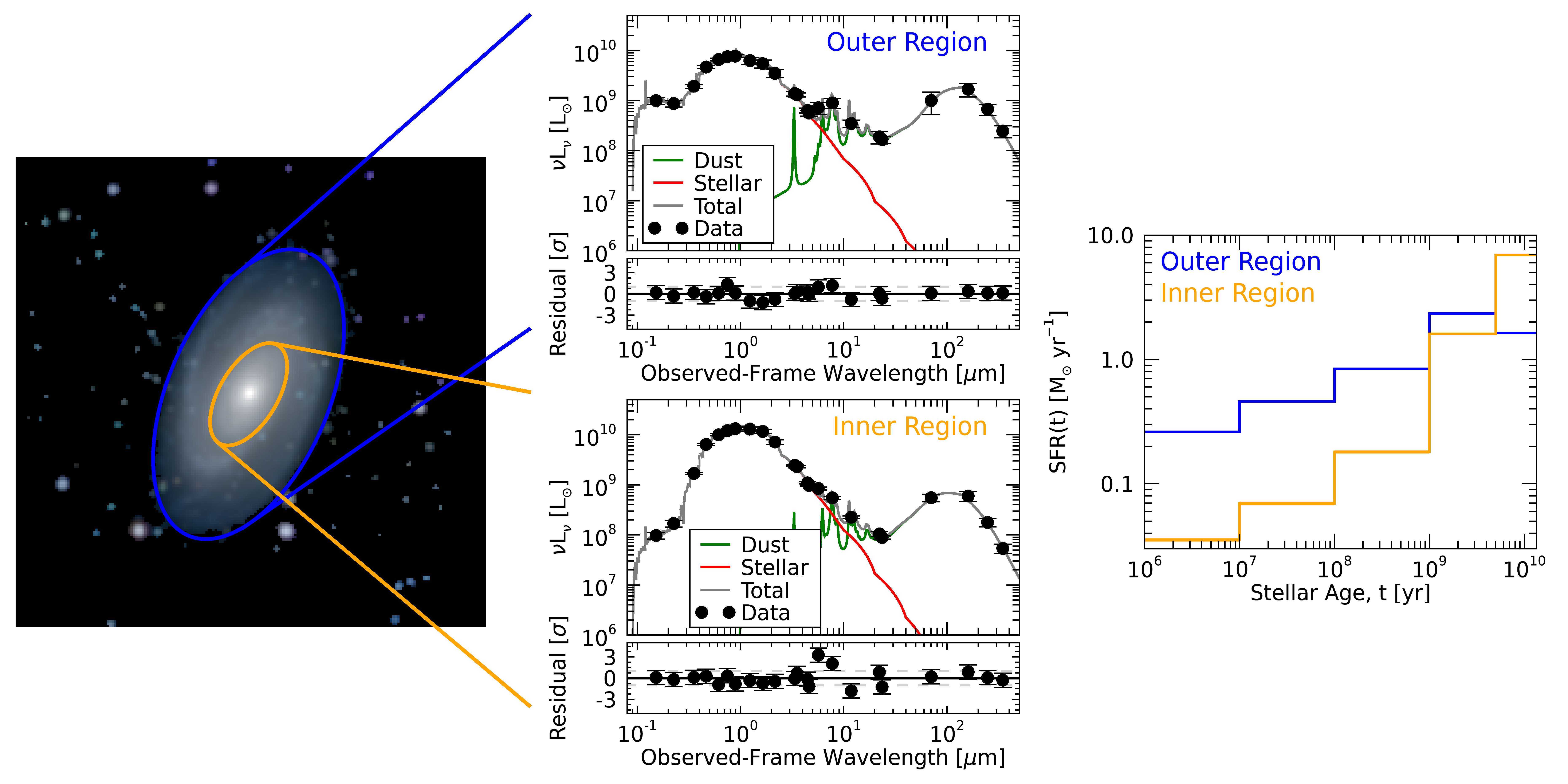
Neat, as we inferred from the maps of the physical properties above, the outer region has comparatively increased UV emission and decreased NIR emission in the observed SED, which is being distinguished by the fit as an overall younger population compared to the inner region. This younger population can be seen as a larger (smaller) SFR in the younger (older) age bins of the SFH.

Finally, to tie in our MPFIT results, lets re-plot the maps of the physical properties to see how they compare. First, we will need to map the results from the post-processing of each SED to its associated pixel.

; We need to match each SED_ID from the result back to the map.
map_idc = lonarr(nsed)
for i=0, nsed-1 do map_idc[i] = where(m81_map eq float(strtrim(results_mpfit[i].sed_id, 2)))

; Make a blank map to fill in with the results values.
sfr_map_mpfit = replicate(!values.f_NaN, map_size)
; The SFR of the last 100 My is the weighted sum of the first two bins (0-10 and 10-100 Myr).
;   The bin index is the first dimension.
sfr_map_mpfit[map_idc] = (results_mpfit.psi)[0, *] * 0.1 + (results_mpfit.psi)[1, *] * 0.9

mass_map_mpfit = replicate(!values.f_NaN, map_size)
mass_map_mpfit[map_idc] = results_mpfit.mstar

tauv_diff_map_mpfit = replicate(!values.f_NaN, map_size)
tauv_diff_map_mpfit[map_idc] = results_mpfit.tauv_diff

ltir_map_mpfit = replicate(!values.f_NaN, map_size)
ltir_map_mpfit[map_idc] = results_mpfit.ltir

pvalue_map_mpfit = replicate(!values.f_NaN, map_size)
pvalue_map_mpfit[map_idc] = max(results_mpfit.pvalue, dim=1)

Again, let’s crop these maps to remove the padded region surrounding the B-band ellipse.

; Crop each image to only include the B-band region.
sfr_map_mpfit = sfr_map_mpfit[mask_bounds_idc[0, 0]:mask_bounds_idc[1, 0], *]
sfr_map_mpfit = sfr_map_mpfit[*, mask_bounds_idc[0, 1]:mask_bounds_idc[1, 1]]

mass_map_mpfit = mass_map_mpfit[mask_bounds_idc[0, 0]:mask_bounds_idc[1, 0], *]
mass_map_mpfit = mass_map_mpfit[*, mask_bounds_idc[0, 1]:mask_bounds_idc[1, 1]]

tauv_diff_map_mpfit = tauv_diff_map_mpfit[mask_bounds_idc[0, 0]:mask_bounds_idc[1, 0], *]
tauv_diff_map_mpfit = tauv_diff_map_mpfit[*, mask_bounds_idc[0, 1]:mask_bounds_idc[1, 1]]

ltir_map_mpfit = ltir_map_mpfit[mask_bounds_idc[0, 0]:mask_bounds_idc[1, 0], *]
ltir_map_mpfit = ltir_map_mpfit[*, mask_bounds_idc[0, 1]:mask_bounds_idc[1, 1]]

pvalue_map_mpfit = pvalue_map_mpfit[mask_bounds_idc[0, 0]:mask_bounds_idc[1, 0], *]
pvalue_map_mpfit = pvalue_map_mpfit[*, mask_bounds_idc[0, 1]:mask_bounds_idc[1, 1]]

Finally, let’s scale the images to have the same minimum and maximum values as the MCMC images to keep the colorbars the same.

keep_nan = where(~finite(sfr_map_mpfit))

; The > and < operators set values below/above that value to the specified value
pvalue_map_mpfit = 10^(((alog10(pvalue_map_mpfit) > min((alog10(pvalue_map))[where(finite(alog10(pvalue_map)))])) < $
                   max((alog10(pvalue_map))[where(finite(alog10(pvalue_map)))])))
sfr_map_mpfit  = ((sfr_map_mpfit > min(sfr_map)) < max(sfr_map))
mass_map_mpfit = ((mass_map_mpfit > min(mass_map)) < max(mass_map))
ssfr_map_mpfit = 10^((alog10(sfr_map_mpfit/mass_map_mpfit)   > (min(alog10(sfr_map/mass_map)))) < $
                  max(alog10(sfr_map/mass_map)))
tauv_diff_map_mpfit   = ((tauv_diff_map_mpfit > min(tauv_diff_map)) < max(tauv_diff_map))
ltir_map_mpfit   = ((ltir_map_mpfit > min(ltir_map)) < max(ltir_map))

; The > and < operators override NaNs, set the NaN pixels back to NaN
pvalue_map_mpfit[keep_nan] = !values.D_NaN
sfr_map_mpfit[keep_nan] = !values.D_NaN
mass_map_mpfit[keep_nan]   = !values.D_NaN
ssfr_map_mpfit[keep_nan]   = !values.D_NaN
tauv_diff_map_mpfit[keep_nan]   = !values.D_NaN
ltir_map_mpfit[keep_nan]   = !values.D_NaN

Now time to plot these images!

; Plotting is simple with our figure script
fig = m81_maps(sfr_map_mpfit, mass_map_mpfit, ssfr_map_mpfit, tauv_diff_map_mpfit, ltir_map_mpfit, pvalue_map_mpfit)

From these panels, we can see that the stellar mass, \(\tau_{{\rm DIFF}, V}\), and \(L_{\rm TIR}\) images are very similar to the MCMC results. The main difference is in the SFR and sSFR images. The differences in these images is mainly the lack of smoothness. This loss of smoothness is primarily due to the usage of the best fit rather than medians of the posterior as the pixel values, since the median of the posterior is rarely the same as the best-fit solution. Additionally, the central region can be seen to have best-fit solutions that are suggesting zero SFR in the MPFIT image. These zero values from MPFIT are not unexpected, since SFR posterior distributions from the MCMC algorithm generally show upper limits, with the maximum probability coinciding with zero.