Stellar X-ray Emission in the Edge-on Galaxy NGC 4631#
The following example shows how how X-rays emitted from the stellar binary population along with inclination-dependent attenuation can be used to help constrain the SFR of the edge-on galaxy, NGC 4631.
Data#
For this example we will include 4 bands of X-ray photometry (0.5–1, 1–2, 2–4, and 4–7 keV) when fitting with an X-ray model. This photometry was generated from the Chandra ACIS-I data (ObsID 797) using the procedures detailed in Section~3.2 of Lehmer et al. (2019). This method did not generate uncertainties on the X-ray fluxes. Therefore, we assume a base 10% uncertainty for each band. Additionally, we assume a Galactic HI column density of \(N_H = 1.29 \times 10^{20}\ {\rm cm}^{-2}\).
For the UV-to-submm photometry, we utilize the data for NGC 4631 from Table 2 of Dale et al. (2017), which we correct for Galactic extinction using their listed values in Tables 1 and 2.
The relevant data files, with and without X-ray data, can be found in examples/inclined_NGC_4631/ as
ngc4631_dale17+xrays_photometry.fits and ngc4631_dale17_photometry.fits, respectively.
Configuration#
To show the effects of including X-rays and inclination-dependence in this example, we want to model
the SED four different ways, using the permutations of including and excluding stellar
X-ray Emission with the base Calzetti and Doore+21 Dust Attenuation curves.
To model the SED four ways, we first change the below lines of the configuration files in
examples/inclined_NGC_4631/Calz+Xrays/, examples/inclined_NGC_4631/Calz/, examples/inclined_NGC_4631/Doore+Xrays/,
and examples/inclined_NGC_4631/Doore/ from the defaults to the configuration settings in common
between the the four models.
Common Settings#
We add 5% model uncertainty
91MODEL_UNC: 0.05d0 ,$
As for the dust emission model, we limit initialization of \(U_{\rm min}\) and \(\gamma\) to lower values than the default, since nearby galaxies like NGC 4631 typically have \(U_{\rm min} < 5\) and \(\gamma \approx 0.01\) (Dale et al. 2017).
341UMIN:    {Prior: 'uniform'                            ,$
342          Prior_arg: [0.1d, 25.d]                     ,$
343          Initialization_range: [0.1d, 5.d]            $
344          }                                           ,$
374GAMMA:   {Prior: 'uniform'                            ,$
375          Prior_arg: [0.0d, 1.0d]                     ,$
376          Initialization_range: [0.0d, 0.1d]           $
377          }                                           ,$
For the post-processing setting of the MCMC algorithm, we increase the number of final elements to 2000:
643FINAL_CHAIN_LENGTH: 2000 ,$
Calzetti Attenuation#
For the two models using the Calzetti attenuation, we will adjust the initializations on \(\tau_V\) to smaller values, since the average attenuation should generally be low.
220TAUV:      {Prior: 'uniform'                          ,$
221            Prior_arg: [0.0d, 10.0d]                  ,$
222            Initialization_range: [0.0d, 1.0d]         $
223            }                                         ,$
We will also decrease the number of MCMC trials required to \(10^4\), since the base Calzetti models (even with stellar X-ray emission) tend to converge quickly.
539NTRIALS: 1e4 ,$
Doore+21 Attenuation#
For the two models using the inclination-dependent Doore+21 attenuation, we will first set them to use this attenuation curve.
211ATTEN_CURVE: 'DOORE21' ,$
Next, we will adjust the initialization range for \(\tau_B^f\) to lower values, since, like the Calzetti attenuation, we expect lower attenuation.
269TAUB_F:    {Prior: 'uniform'                          ,$
270            Prior_arg: [0.0d, 8.0d]                   ,$
271            Initialization_range: [0.0d, 4.0d]         $
272            }                                         ,$
Most importantly, we will then set \(\cos i\) to have a tabulated prior using the Monte Carlo (MC)
method described in Section 3 of Doore et al. 2021.
This prior will be placed in the examples/inclined_NGC_4631/ directory of Lightning. So, we will set the path to the
absolute path using the !lightning_dir system variable created when you first built Lightning.
289COSI:      {Prior: 'tabulated'                               ,$
290            Prior_arg: [!lightning_dir+'examples/NGC_4631/'] ,$
291            Initialization_range: [0.005d, 0.2d]              $
292            }                                                ,$
To generate this prior, we have created a function (inclination_pdf.pro) that performs the MC simulation
with the inputs of the axis ratio and its uncertainty. The function also normalizes the distribution to have
a total area of 1 as required by Lightning. For the axis ratio, we use the B-band ellipse values from the
HyperLeda database, since they have associated uncertainties. The prior
generation can then be done with:
cd, !lightning_dir + 'examples/NGC_4631/'

; Axis ratio gathered from HyperLeda database.
logr25 = 0.82  ; logr25 is the axis ratio of the isophote (decimal logarithm of the ratio of the lengths of major to minor axes).
elogr25 = 0.05 ; error on logr25

; Convert from logr25 to q
q = 10.d^(-1.d * logr25) ; axis ratio is q = b/a, negative flips ratio from major/minor to minor/major.
q_err = q * alog(10.d) * elogr25

; Perform the Monte Carlo (MC) simulation
inclination_pdf, q, q_err, 'gamma_eps_distribution_tables/', inc_bins, inc_pdf, units='cosi'

; Now add the results from the MC simulation into the prior structure.
;   Also, let's smooth the pdf some since it is randomly generated.
prior = {cosi_values: inc_bins, cosi_pdf: smooth(inc_pdf, 5)}

; Save the structure to the correctly named FITS file.
mwrfits, prior, 'tabulated_prior_NGC_4631.fits', /create
Additionally, let’s plot this prior to make sure we are getting a distribution that strongly favors an edge-on view:
plt = plot(1 - prior.cosi_values, $
           prior.cosi_pdf, $
           xtitle='1 - cos(i)', $
           ytitle='Probability', $
           thick=2)
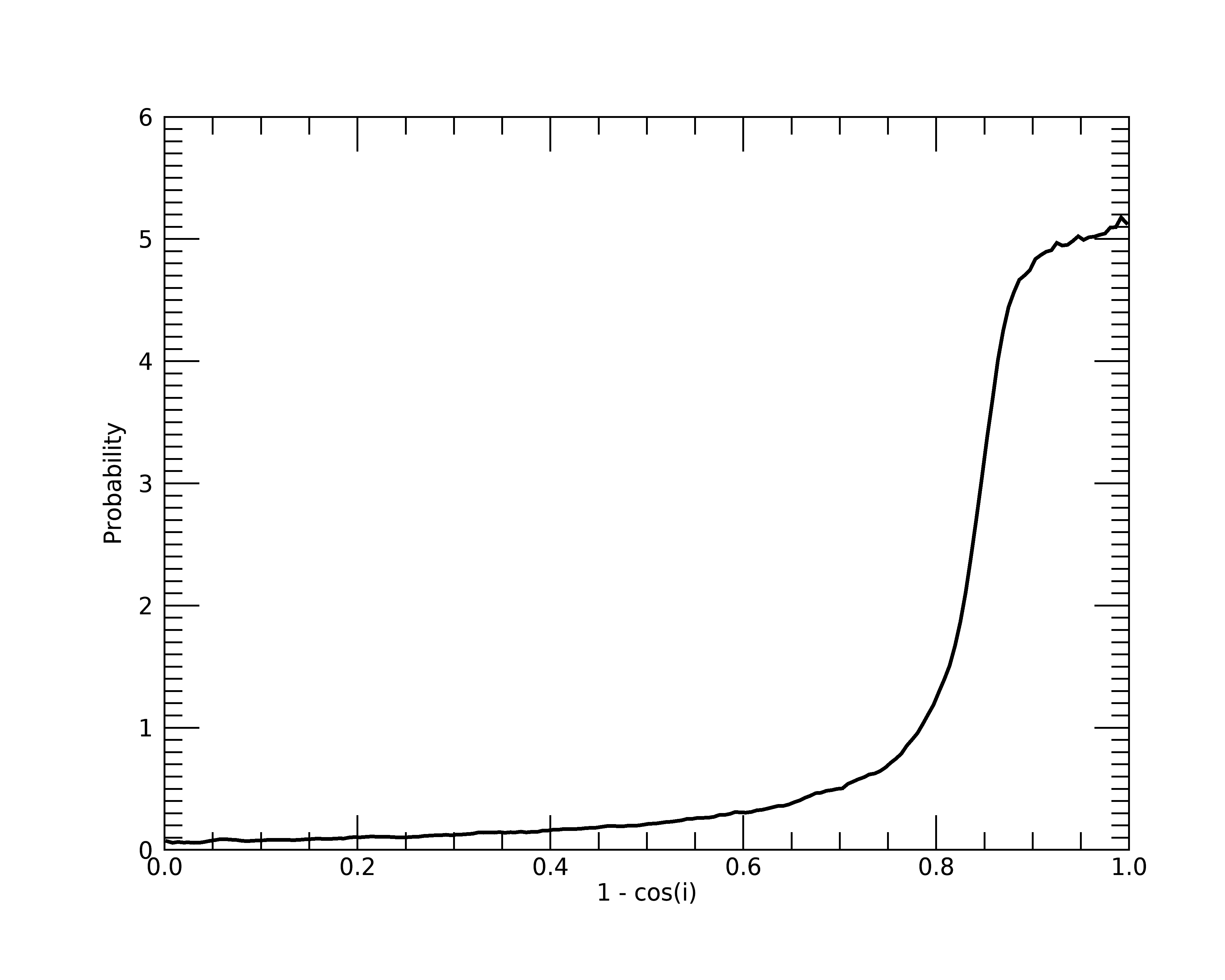
Great, as we can see, the probability distribution is skewed to values with \(1 - \cos i > 0.8\), which corresponds to \(i > 78^\circ\). Therefore, this distribution highly favors the edge-on views as we want.
Going back to the configuration, we will fix the bulge-to-disk ratio of the Doore+21 attenuation to 0, since we are assuming NGC 4631 is disk dominated.
299B_TO_D:    {Prior: 'fixed'                            ,$
300            Prior_arg: [0.0d]                         ,$
301            Initialization_range: [0.0d, 0.d0]         $
302            }                                         ,$
We will then increase the number of MCMC trials required to \(5 \times 10^4\), since the Doore+21 models can take a while to properly converge.
539NTRIALS: 5e4 ,$
X-ray Fit#
For the two models using X-ray emission, we additionally modify the following settings. First, we turn on the X-ray emission module:
415XRAY_EMISSION: 1 ,$
We then set Lightning to expect our X-ray data in fluxes and make sure to turn off the X-ray AGN model:
422XRAY_UNIT: 'FLUX' ,$
450XRAY_AGN_MODEL: 'NONE' ,$
Individual Fits#
Finally, for each of the configurations, we need to update their output file names. For the Calzetti
fit with X-rays (examples/inclined_NGC_4631/Calz+Xrays/lightning_configure.pro), we will name the output:
71OUTPUT_FILENAME: 'calz_with_xrays' ,$
For the Calzetti without X-rays (examples/inclined_NGC_4631/Calz/lightning_configure.pro):
71OUTPUT_FILENAME: 'calz_no_xrays' ,$
For the Doore+21 with X-rays (examples/inclined_NGC_4631/Doore+Xrays/lightning_configure.pro):
71OUTPUT_FILENAME: 'doore_with_xrays' ,$
And for the Doore+21 without X-rays (examples/inclined_NGC_4631/Doore/lightning_configure.pro):
71OUTPUT_FILENAME: 'doore_no_xrays' ,$
Running Lightning#
Note
The IDL code snippets below (and the inclination prior ones above) are also available
in batch file format, as examples/inclined_NGC_4631/ngc4631_batch.pro.
Now that we have set up the configurations, we are ready to run Lightning for each of the
models. Before, we do that we need to quickly copy the input data into each fitting
directory (e.g., examples/inclined_NGC_4631/Calz+Xrays/).
; Copy the photometry into the fitting directories
file_copy, 'ngc4631_dale17_photometry.fits', 'Calz/', /allow_same
file_copy, 'ngc4631_dale17_photometry.fits', 'Doore/', /allow_same
file_copy, 'ngc4631_dale17+xrays_photometry.fits', 'Calz+Xrays/', /allow_same
file_copy, 'ngc4631_dale17+xrays_photometry.fits', 'Doore+Xrays/', /allow_same
Additionally, we have pre-compiled the needed \(L_{\rm bol}^{\rm abs}\) table for the Doore+21 model to save time during fitting, as generating this table can take a while on machines with < 10GB of RAM. So, we need to copy it into the Doore+21 fitting directories.
; Copy the Lbol_abs table directory into the Doore21 fitting directories
file_mkdir, ['Doore+Xrays/', 'Doore/'] + 'lightning_output/'
file_copy, replicate('doore21_Lbol_abs_table/', 2), $
           ['Doore+Xrays/', 'Doore/'] + 'lightning_output/', /allow_same, /recursive
Now, we can fit all of the models to the SED with:
restore, !lightning_dir + 'lightning.sav'

lightning, 'Calz/ngc4631_dale17_photometry.fits'
lightning, 'Calz+Xrays/ngc4631_dale17+xrays_photometry.fits'
lightning, 'Doore/ngc4631_dale17_photometry.fits'
lightning, 'Doore+Xrays/ngc4631_dale17+xrays_photometry.fits'
With the MCMC configuration we’ve selected for the Calzetti fits, this may take around 20–25 minutes each on a simple laptop CPU (we ran it on a ca. 2016 1.2 GHz Intel Core m5). For the increased MCMC trials of the Doore+21 fits, it may take around 1.5–2 hours each. We note that you can run these fits simultaneously in separate IDL sessions.
Analysis#
Once the fits finish, Lightning will automatically create post-processed files for us containing the results.
; Read in each post-processed files
calz    = mrdfits('Calz/lightning_output/calz_no_xrays.fits.gz', 1)
calz_x  = mrdfits('Calz+Xrays/lightning_output/calz_with_xrays.fits.gz', 1)
doore   = mrdfits('Doore/lightning_output/doore_no_xrays.fits.gz', 1)
doore_x = mrdfits('Doore+Xrays/lightning_output/doore_with_xrays.fits.gz', 1)
Convergence#
As always, we need to first check each of our fits for convergence.
; Let's check each fit, if any, did not reach convergence by all our metrics.
print, '//Convergence Checks//'
print, '//Convergence for the Calzetti (no X-rays) fit//'
print, 'Mean acceptance fraction: ', strtrim(mean(calz.acceptance_frac), 2)
print, 'Convergence flag: ', strtrim(calz.convergence_flag, 2)
; Include the short chain flag since we had lightning automatically choose the burn-in and thinning
print, 'Short chain flag: ', strtrim(calz.short_chain_flag, 2)

print, ''
print, '//Convergence for the Calzetti with X-rays fit//'
print, 'Mean acceptance fraction: ', strtrim(mean(calz_x.acceptance_frac), 2)
print, 'Convergence flag: ', strtrim(calz_x.convergence_flag, 2)
print, 'Short chain flag: ', strtrim(calz_x.short_chain_flag, 2)

print, ''
print, '//Convergence for the Doore+21 (no X-rays) fit//'
print, 'Mean acceptance fraction: ', strtrim(mean(doore.acceptance_frac), 2)
print, 'Convergence flag: ', strtrim(doore.convergence_flag, 2)
print, 'Short chain flag: ', strtrim(doore.short_chain_flag, 2)

print, ''
print, '//Convergence for the Doore+21 with X-rays  fit//'
print, 'Mean acceptance fraction: ', strtrim(mean(doore_x.acceptance_frac), 2)
print, 'Convergence flag: ', strtrim(doore_x.convergence_flag, 2)
print, 'Short chain flag: ', strtrim(doore_x.short_chain_flag, 2)
//Convergence Checks//
//Convergence for the Calzetti (no X-rays) fit//
Mean acceptance fraction: 0.36408533
Convergence flag: 0
Short chain flag: 0

//Convergence for the Calzetti with X-rays fit//
Mean acceptance fraction: 0.35554533
Convergence flag: 0
Short chain flag: 0

//Convergence for the Doore+21 (no X-rays) fit//
Mean acceptance fraction: 0.28195600
Convergence flag: 1
Short chain flag: 0

//Convergence for the Doore+21 with X-rays  fit//
Mean acceptance fraction: 0.28607467
Convergence flag: 0
Short chain flag: 0
Great, as we can see, all fits had enough independent trials to create the 2000 samples we
wanted (short_chain_flag = 0). Also, all of the fits converged except the one for the
Doore+21 attenuation without X-rays. Let’s separate out its autocorrelation time metric and
acceptance fraction metrics to see which is indicating potentially failed convergence.
print, '//Detailed Convergence Checks//'
print, 'Number of parameters with high autocorrelation times: ', strtrim(total(doore.autocorr_flag), 2)
print, 'Number of walkers with low acceptance fractions: ', strtrim(total(doore.acceptance_flag), 2)
//Detailed Convergence Checks//
Number of parameters with high autocorrelation times: 1.00000
Number of walkers with low acceptance fractions: 0.00000
Okay, so the acceptance fractions are good, and only one parameter has a high autocorrelation
time. Let’s check what parameter this is and how it compares to our factor of 50 threshold for
considering convergence (i.e., NTRIALS/AUTOCORR_TIME should be ~50).
print, '//Autocorrelation Time Checks//'
print, 'Parameter with high autocorrelation time: ', $
       strtrim((doore.parameter_names)[where(doore.autocorr_flag eq 1, /null)], 2)
print, 'Ratio of Ntrials to autocorr_time: ', $
       strtrim(5e4/((doore.autocorr_time)[where(doore.autocorr_flag eq 1, /null)]), 2)
//Autocorrelation Time Checks//
Parameter with high autocorrelation time:  COSI
Ratio of Ntrials to autocorr_time:  48.923960
This is good to see. The “problem” parameter is the inclination, which we expected either it or \(\tau_B^f\) to be. Additionally, we can see that it is just barely below our default threshold of 50. Since we want a value of ~50, this is close enough, and we can be confident that our autocorrelation time for the inclination is accurate. Therefore, our solution has converged.
Figure#
Now that we have confirmed convergence, we will make a figure to see how the SFRs from the fits compare.
To do this, we will plot the posterior of each SFR of the last 100 My and the best-fit spectra to the
SED. We have prepared a function for this: ngc4631_plots.pro.
; Load the cgs constants, as the plotting script needs them
lightning_constants

; Plotting is simple with our figure script
fig = ngc4631_plots(calz, calz_x, doore, doore_x)
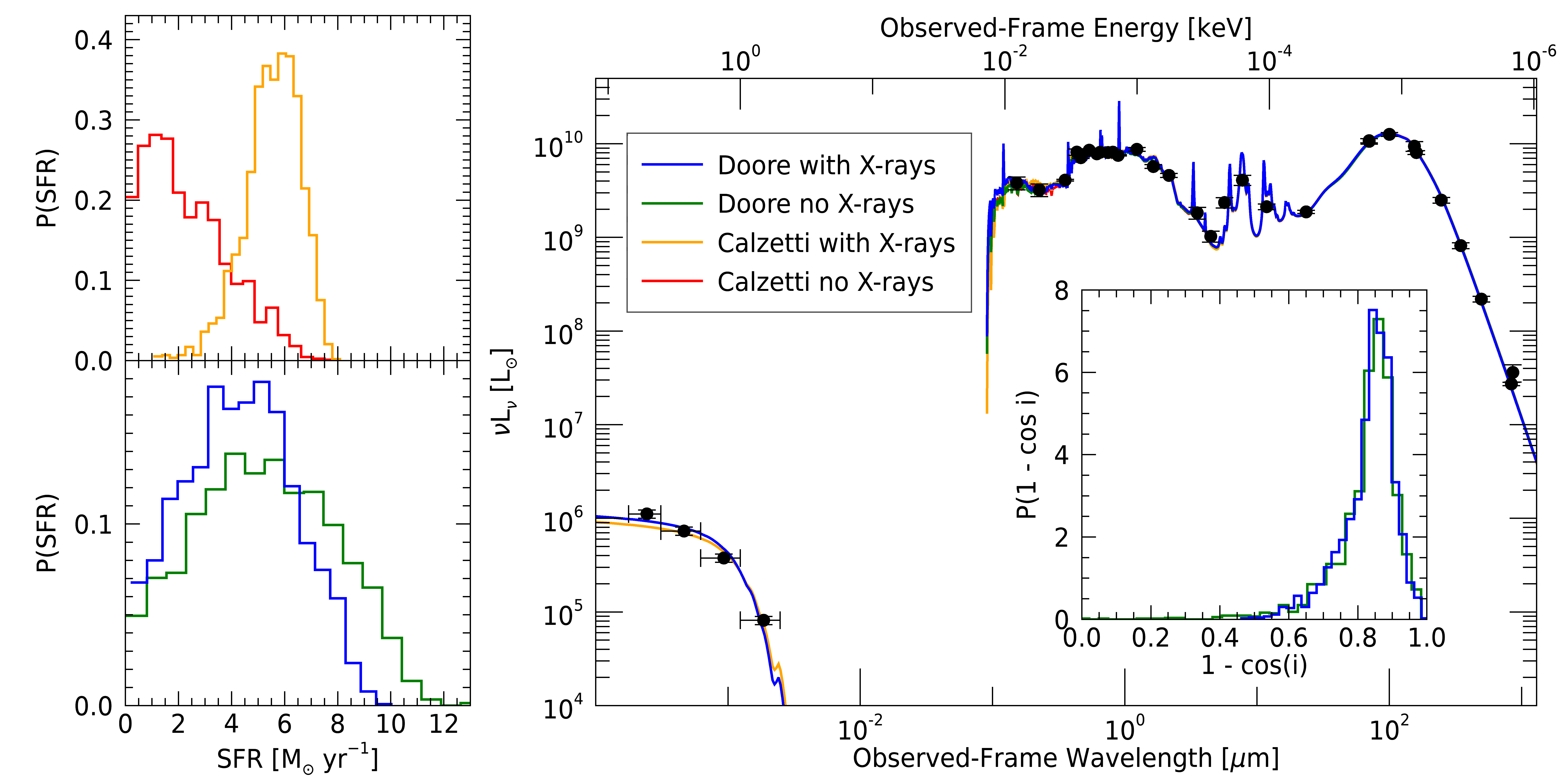
From the plot, each of the four models’ SFRs can be seen to have general agreement, with the Calzetti models having stronger variation when including the X-rays compared to the Doore+21 models. Since the Calzetti attenuation model assumes a uniform spherical distribution of stars and dust, it is too simplistic for edge-on galaxies. Therefore, by including the inclination dependences of the Doore+21 models, we can get a more accurate estimate of the SFR, with the inclusion of the X-rays increasing the precision as we would expect. Further, the X-ray data rules out some higher SFR solutions in both cases (i.e., \({\rm SFR} > 8\ M_\odot\ {\rm yr}^{-1}\)), as they become more unlikely with the X-ray data constraint.